RNAseq-R-tidyverse

Introduction

This material presents how to perform analysis of RNA sequencing data following the tidy data paradigm (Wickham et al. 2014). The tidy data paradigm provides a standard way to organise data values within a dataset, where each variable is a column, each observation is a row, and data is manipulated using an easy-to-understand vocabulary. Most importantly, the data structure remains consistent across manipulation and analysis functions.

This can be achieved for RNA sequencing data with the tidybulk(Mangiola et al. 2021), tidyHeatmap (Mangiola and Papenfuss 2020) and tidyverse (Wickham et al. 2019) packages. The tidybulk package provides a tidy data structure and a modular framework for bulk transcriptional analyses. tidyHeatmap provides a tidy implementation of ComplexHeatmap. These packages are part of the tidytranscriptomics suite that introduces a tidy approach to RNA sequencing data representation and analysis

Acknowledgements

This material was adapted from an R for RNA sequencing workshop first run here.

Setting up the data

First, let’s load all the packages we will need to analyse the data.

Note: you should load the tidybulk library after the tidyverse core packages for best integration.

# load libraries

library(tibble)
library(dplyr)
library(tidyr)
library(readr)
library(stringr)
library(ggplot2)
library(plotly)
library(ggrepel)
library(EGSEA)
library(tidyHeatmap)
library(tidybulk)

Plot settings. Set the colours and theme we will use for our plots.

# Use colourblind-friendly colours
friendly_cols <- c("#999999", "#E69F00", "#56B4E9", "#009E73", "#F0E442", "#0072B2", "#D55E00", "#CC79A7")

# Set theme
custom_theme <-
  list(
    scale_fill_manual(values = friendly_cols),
    scale_color_manual(values = friendly_cols),
    theme_bw() +
      theme(
        panel.border = element_blank(),
        axis.line = element_line(),
        panel.grid.major = element_line(size = 0.2),
        panel.grid.minor = element_line(size = 0.1),
        text = element_text(size = 12),
        legend.position = "bottom",
        strip.background = element_blank(),
        axis.title.x = element_text(margin = margin(t = 10, r = 10, b = 10, l = 10)),
        axis.title.y = element_text(margin = margin(t = 10, r = 10, b = 10, l = 10)),
        axis.text.x = element_text(angle = 30, hjust = 1, vjust = 1)
      )
  )

Mouse mammary gland dataset

Here we will perform RNA-Seq analysis using data from a breast cancer research study, from the paper by Fu et al. 2015, GEO code GSE60450. This study examined gene expression in basal and luminal cells from mice at different stages of mammary gland development (virgin, pregnant and lactating). There are 2 samples per group and 6 groups, 12 samples in total.

Importing the data

# import RNA-seq counts
seqdata <- read_tsv("https://ndownloader.figshare.com/files/5057929?private_link=1d788fd384d33e913a2a")
#> Rows: 27179 Columns: 14
#> ── Column specification ────────────────────────────────────────────────────────
#> Delimiter: "\t"
#> dbl (14): EntrezGeneID, Length, MCL1-DG_BC2CTUACXX_ACTTGA_L002_R1, MCL1-DH_B...
#> 
#> ℹ Use `spec()` to retrieve the full column specification for this data.
#> ℹ Specify the column types or set `show_col_types = FALSE` to quiet this message.

# import sample information
sampleinfo <- read_tsv("https://ndownloader.figshare.com/files/5999832?private_link=1d788fd384d33e913a2a")
#> Rows: 12 Columns: 4
#> ── Column specification ────────────────────────────────────────────────────────
#> Delimiter: "\t"
#> chr (4): FileName, SampleName, CellType, Status
#> 
#> ℹ Use `spec()` to retrieve the full column specification for this data.
#> ℹ Specify the column types or set `show_col_types = FALSE` to quiet this message.

Take a look at the data.

seqdata
#> # A tibble: 27,179 × 14
#>    EntrezGeneID Length `MCL1-DG_BC2CTUACXX_A…` `MCL1-DH_BC2CT…` `MCL1-DI_BC2CT…`
#>           <dbl>  <dbl>                   <dbl>            <dbl>            <dbl>
#>  1       497097   3634                     438              300               65
#>  2    100503874   3259                       1                0                1
#>  3    100038431   1634                       0                0                0
#>  4        19888   9747                       1                1                0
#>  5        20671   3130                     106              182               82
#>  6        27395   4203                     309              234              337
#>  7        18777   2433                     652              515              948
#>  8    100503730    799                       0                1                0
#>  9        21399   2847                    1604             1495             1721
#> 10        58175   2241                       4                2               14
#> # … with 27,169 more rows, and 9 more variables:
#> #   `MCL1-DJ_BC2CTUACXX_CGATGT_L002_R1` <dbl>,
#> #   `MCL1-DK_BC2CTUACXX_TTAGGC_L002_R1` <dbl>,
#> #   `MCL1-DL_BC2CTUACXX_ATCACG_L002_R1` <dbl>,
#> #   `MCL1-LA_BC2CTUACXX_GATCAG_L001_R1` <dbl>,
#> #   `MCL1-LB_BC2CTUACXX_TGACCA_L001_R1` <dbl>,
#> #   `MCL1-LC_BC2CTUACXX_GCCAAT_L001_R1` <dbl>, …

In the seqdata object, the first column contains the Entrez gene identifier, the second column contains the gene length and the rest of the columns contain the gene transcription abundance for each sample. The abundance is the number of reads aligning to the gene in each experimental sample.

Format the data

We first convert the counts into long format (tidy format) so we can join to the sample information and also use with ggplot and other tidyverse functions.

In this workshop we make use of the tidyverse pipe %>%. This ‘pipes’ the output from the command on the left into the command on the right/below. Using the pipe is not essential but it can make the steps clearer and easier to see. For more details on the pipe see here.

counts_long <- seqdata %>% pivot_longer(cols = starts_with("MCL"), names_to = "sample", values_to = "counts")

# take a look
counts_long
#> # A tibble: 326,148 × 4
#>    EntrezGeneID Length sample                            counts
#>           <dbl>  <dbl> <chr>                              <dbl>
#>  1       497097   3634 MCL1-DG_BC2CTUACXX_ACTTGA_L002_R1    438
#>  2       497097   3634 MCL1-DH_BC2CTUACXX_CAGATC_L002_R1    300
#>  3       497097   3634 MCL1-DI_BC2CTUACXX_ACAGTG_L002_R1     65
#>  4       497097   3634 MCL1-DJ_BC2CTUACXX_CGATGT_L002_R1    237
#>  5       497097   3634 MCL1-DK_BC2CTUACXX_TTAGGC_L002_R1    354
#>  6       497097   3634 MCL1-DL_BC2CTUACXX_ATCACG_L002_R1    287
#>  7       497097   3634 MCL1-LA_BC2CTUACXX_GATCAG_L001_R1      0
#>  8       497097   3634 MCL1-LB_BC2CTUACXX_TGACCA_L001_R1      0
#>  9       497097   3634 MCL1-LC_BC2CTUACXX_GCCAAT_L001_R1      0
#> 10       497097   3634 MCL1-LD_BC2CTUACXX_GGCTAC_L001_R1      0
#> # … with 326,138 more rows

We can shorten the sample names to just the relevant information, the first 7 characters.

counts_formatted <- counts_long %>% mutate(sample_name=str_extract(sample, "MCL1-.."))

# take a look
counts_formatted
#> # A tibble: 326,148 × 5
#>    EntrezGeneID Length sample                            counts sample_name
#>           <dbl>  <dbl> <chr>                              <dbl> <chr>      
#>  1       497097   3634 MCL1-DG_BC2CTUACXX_ACTTGA_L002_R1    438 MCL1-DG    
#>  2       497097   3634 MCL1-DH_BC2CTUACXX_CAGATC_L002_R1    300 MCL1-DH    
#>  3       497097   3634 MCL1-DI_BC2CTUACXX_ACAGTG_L002_R1     65 MCL1-DI    
#>  4       497097   3634 MCL1-DJ_BC2CTUACXX_CGATGT_L002_R1    237 MCL1-DJ    
#>  5       497097   3634 MCL1-DK_BC2CTUACXX_TTAGGC_L002_R1    354 MCL1-DK    
#>  6       497097   3634 MCL1-DL_BC2CTUACXX_ATCACG_L002_R1    287 MCL1-DL    
#>  7       497097   3634 MCL1-LA_BC2CTUACXX_GATCAG_L001_R1      0 MCL1-LA    
#>  8       497097   3634 MCL1-LB_BC2CTUACXX_TGACCA_L001_R1      0 MCL1-LB    
#>  9       497097   3634 MCL1-LC_BC2CTUACXX_GCCAAT_L001_R1      0 MCL1-LC    
#> 10       497097   3634 MCL1-LD_BC2CTUACXX_GGCTAC_L001_R1      0 MCL1-LD    
#> # … with 326,138 more rows

Now let’s take a look at the sample information table.

sampleinfo
#> # A tibble: 12 × 4
#>    FileName                          SampleName CellType Status  
#>    <chr>                             <chr>      <chr>    <chr>   
#>  1 MCL1.DG_BC2CTUACXX_ACTTGA_L002_R1 MCL1.DG    basal    virgin  
#>  2 MCL1.DH_BC2CTUACXX_CAGATC_L002_R1 MCL1.DH    basal    virgin  
#>  3 MCL1.DI_BC2CTUACXX_ACAGTG_L002_R1 MCL1.DI    basal    pregnant
#>  4 MCL1.DJ_BC2CTUACXX_CGATGT_L002_R1 MCL1.DJ    basal    pregnant
#>  5 MCL1.DK_BC2CTUACXX_TTAGGC_L002_R1 MCL1.DK    basal    lactate 
#>  6 MCL1.DL_BC2CTUACXX_ATCACG_L002_R1 MCL1.DL    basal    lactate 
#>  7 MCL1.LA_BC2CTUACXX_GATCAG_L001_R1 MCL1.LA    luminal  virgin  
#>  8 MCL1.LB_BC2CTUACXX_TGACCA_L001_R1 MCL1.LB    luminal  virgin  
#>  9 MCL1.LC_BC2CTUACXX_GCCAAT_L001_R1 MCL1.LC    luminal  pregnant
#> 10 MCL1.LD_BC2CTUACXX_GGCTAC_L001_R1 MCL1.LD    luminal  pregnant
#> 11 MCL1.LE_BC2CTUACXX_TAGCTT_L001_R1 MCL1.LE    luminal  lactate 
#> 12 MCL1.LF_BC2CTUACXX_CTTGTA_L001_R1 MCL1.LF    luminal  lactate

The CellType column tells us whether the samples are from basal or luminal cells and the Status column tells us what stage of mouse mammary gland development they are from.

We’ll create a column containing the groups we’ll be examining e.g. basal.pregnant and basal.lactate by joining the CellType and Status columns using unite. We’ll use mutate to edit the sample id so we can join to the counts.

sampleinfo_formatted <- sampleinfo %>%
    
    # make column called Group by combining the CellType and Status columns
    unite("Group", CellType:Status, sep=".", remove=FALSE) %>%
    
    # replace the . in the SampleName with - so can join to counts
    mutate(sample_name=str_replace(SampleName, "\\.", "-"))

# take a look
sampleinfo_formatted 
#> # A tibble: 12 × 6
#>    FileName                         SampleName Group CellType Status sample_name
#>    <chr>                            <chr>      <chr> <chr>    <chr>  <chr>      
#>  1 MCL1.DG_BC2CTUACXX_ACTTGA_L002_… MCL1.DG    basa… basal    virgin MCL1-DG    
#>  2 MCL1.DH_BC2CTUACXX_CAGATC_L002_… MCL1.DH    basa… basal    virgin MCL1-DH    
#>  3 MCL1.DI_BC2CTUACXX_ACAGTG_L002_… MCL1.DI    basa… basal    pregn… MCL1-DI    
#>  4 MCL1.DJ_BC2CTUACXX_CGATGT_L002_… MCL1.DJ    basa… basal    pregn… MCL1-DJ    
#>  5 MCL1.DK_BC2CTUACXX_TTAGGC_L002_… MCL1.DK    basa… basal    lacta… MCL1-DK    
#>  6 MCL1.DL_BC2CTUACXX_ATCACG_L002_… MCL1.DL    basa… basal    lacta… MCL1-DL    
#>  7 MCL1.LA_BC2CTUACXX_GATCAG_L001_… MCL1.LA    lumi… luminal  virgin MCL1-LA    
#>  8 MCL1.LB_BC2CTUACXX_TGACCA_L001_… MCL1.LB    lumi… luminal  virgin MCL1-LB    
#>  9 MCL1.LC_BC2CTUACXX_GCCAAT_L001_… MCL1.LC    lumi… luminal  pregn… MCL1-LC    
#> 10 MCL1.LD_BC2CTUACXX_GGCTAC_L001_… MCL1.LD    lumi… luminal  pregn… MCL1-LD    
#> 11 MCL1.LE_BC2CTUACXX_TAGCTT_L001_… MCL1.LE    lumi… luminal  lacta… MCL1-LE    
#> 12 MCL1.LF_BC2CTUACXX_CTTGTA_L001_… MCL1.LF    lumi… luminal  lacta… MCL1-LF

Adding annotation

To the counts table we can add gene symbols.

counts_annotated <- counts_formatted %>%
    
    mutate(symbol = AnnotationDbi::mapIds(org.Mm.eg.db::org.Mm.eg.db, 
                                          keys = as.character(EntrezGeneID), 
                                          keytype = "ENTREZID", 
                                          column="SYMBOL", 
                                          multiVals = "first"))
#> 'select()' returned 1:1 mapping between keys and columns
# take a look
counts_annotated
#> # A tibble: 326,148 × 6
#>    EntrezGeneID Length sample                          counts sample_name symbol
#>           <dbl>  <dbl> <chr>                            <dbl> <chr>       <chr> 
#>  1       497097   3634 MCL1-DG_BC2CTUACXX_ACTTGA_L002…    438 MCL1-DG     Xkr4  
#>  2       497097   3634 MCL1-DH_BC2CTUACXX_CAGATC_L002…    300 MCL1-DH     Xkr4  
#>  3       497097   3634 MCL1-DI_BC2CTUACXX_ACAGTG_L002…     65 MCL1-DI     Xkr4  
#>  4       497097   3634 MCL1-DJ_BC2CTUACXX_CGATGT_L002…    237 MCL1-DJ     Xkr4  
#>  5       497097   3634 MCL1-DK_BC2CTUACXX_TTAGGC_L002…    354 MCL1-DK     Xkr4  
#>  6       497097   3634 MCL1-DL_BC2CTUACXX_ATCACG_L002…    287 MCL1-DL     Xkr4  
#>  7       497097   3634 MCL1-LA_BC2CTUACXX_GATCAG_L001…      0 MCL1-LA     Xkr4  
#>  8       497097   3634 MCL1-LB_BC2CTUACXX_TGACCA_L001…      0 MCL1-LB     Xkr4  
#>  9       497097   3634 MCL1-LC_BC2CTUACXX_GCCAAT_L001…      0 MCL1-LC     Xkr4  
#> 10       497097   3634 MCL1-LD_BC2CTUACXX_GGCTAC_L001…      0 MCL1-LD     Xkr4  
#> # … with 326,138 more rows

We join the counts and sample information into one table.

counts <- left_join(counts_annotated, sampleinfo_formatted, by = "sample_name")

# take a look
counts
#> # A tibble: 326,148 × 11
#>    EntrezGeneID Length sample      counts sample_name symbol FileName SampleName
#>           <dbl>  <dbl> <chr>        <dbl> <chr>       <chr>  <chr>    <chr>     
#>  1       497097   3634 MCL1-DG_BC…    438 MCL1-DG     Xkr4   MCL1.DG… MCL1.DG   
#>  2       497097   3634 MCL1-DH_BC…    300 MCL1-DH     Xkr4   MCL1.DH… MCL1.DH   
#>  3       497097   3634 MCL1-DI_BC…     65 MCL1-DI     Xkr4   MCL1.DI… MCL1.DI   
#>  4       497097   3634 MCL1-DJ_BC…    237 MCL1-DJ     Xkr4   MCL1.DJ… MCL1.DJ   
#>  5       497097   3634 MCL1-DK_BC…    354 MCL1-DK     Xkr4   MCL1.DK… MCL1.DK   
#>  6       497097   3634 MCL1-DL_BC…    287 MCL1-DL     Xkr4   MCL1.DL… MCL1.DL   
#>  7       497097   3634 MCL1-LA_BC…      0 MCL1-LA     Xkr4   MCL1.LA… MCL1.LA   
#>  8       497097   3634 MCL1-LB_BC…      0 MCL1-LB     Xkr4   MCL1.LB… MCL1.LB   
#>  9       497097   3634 MCL1-LC_BC…      0 MCL1-LC     Xkr4   MCL1.LC… MCL1.LC   
#> 10       497097   3634 MCL1-LD_BC…      0 MCL1-LD     Xkr4   MCL1.LD… MCL1.LD   
#> # … with 326,138 more rows, and 3 more variables: Group <chr>, CellType <chr>,
#> #   Status <chr>

Convert counts to tidybulk tibble

To perform the RNA sequencing analysis steps, we convert into a tidybulk tibble. A tibble is the tidyverse table format.

counts_tt <- counts %>% 
    # convert ids from numeric to character (text) datatype
    mutate(EntrezGeneID = as.character(EntrezGeneID)) %>%
    
    tidybulk(.sample=sample_name, .transcript=EntrezGeneID, .abundance=counts)

# take a look
counts_tt
#> # A tibble: 326,148 × 11
#>    EntrezGeneID Length sample      counts sample_name symbol FileName SampleName
#>    <chr>         <dbl> <chr>        <dbl> <chr>       <chr>  <chr>    <chr>     
#>  1 497097         3634 MCL1-DG_BC…    438 MCL1-DG     Xkr4   MCL1.DG… MCL1.DG   
#>  2 497097         3634 MCL1-DH_BC…    300 MCL1-DH     Xkr4   MCL1.DH… MCL1.DH   
#>  3 497097         3634 MCL1-DI_BC…     65 MCL1-DI     Xkr4   MCL1.DI… MCL1.DI   
#>  4 497097         3634 MCL1-DJ_BC…    237 MCL1-DJ     Xkr4   MCL1.DJ… MCL1.DJ   
#>  5 497097         3634 MCL1-DK_BC…    354 MCL1-DK     Xkr4   MCL1.DK… MCL1.DK   
#>  6 497097         3634 MCL1-DL_BC…    287 MCL1-DL     Xkr4   MCL1.DL… MCL1.DL   
#>  7 497097         3634 MCL1-LA_BC…      0 MCL1-LA     Xkr4   MCL1.LA… MCL1.LA   
#>  8 497097         3634 MCL1-LB_BC…      0 MCL1-LB     Xkr4   MCL1.LB… MCL1.LB   
#>  9 497097         3634 MCL1-LC_BC…      0 MCL1-LC     Xkr4   MCL1.LC… MCL1.LC   
#> 10 497097         3634 MCL1-LD_BC…      0 MCL1-LD     Xkr4   MCL1.LD… MCL1.LD   
#> # … with 326,138 more rows, and 3 more variables: Group <chr>, CellType <chr>,
#> #   Status <chr>

Using this tidybulk tibble we can perform differential expression analysis with the tidybulk package.

Filtering lowly expressed genes

We filter lowly expressed genes using tidybulk keep_abundant or identify_abundant. These functions can use the edgeR filterByExpr function described in (Law et al. 2016) to automatically identify the genes with adequate abundance for differential expression testing. By default, this will keep genes with ~10 counts in a minimum number of samples, the number of the samples in the smallest group. In this dataset the smallest group size is two (we have two replicates for each group). Alternatively, we could use identify_abundant to identify which genes are abundant or not (TRUE/FALSE), rather than just keeping the abundant ones.

# Filtering counts
counts_filtered <- counts_tt %>% keep_abundant(factor_of_interest = Group)

# take a look
counts_filtered
#> # A tibble: 191,628 × 12
#>    EntrezGeneID Length sample      counts sample_name symbol FileName SampleName
#>    <chr>         <dbl> <chr>        <dbl> <chr>       <chr>  <chr>    <chr>     
#>  1 497097         3634 MCL1-DG_BC…    438 MCL1-DG     Xkr4   MCL1.DG… MCL1.DG   
#>  2 497097         3634 MCL1-DH_BC…    300 MCL1-DH     Xkr4   MCL1.DH… MCL1.DH   
#>  3 497097         3634 MCL1-DI_BC…     65 MCL1-DI     Xkr4   MCL1.DI… MCL1.DI   
#>  4 497097         3634 MCL1-DJ_BC…    237 MCL1-DJ     Xkr4   MCL1.DJ… MCL1.DJ   
#>  5 497097         3634 MCL1-DK_BC…    354 MCL1-DK     Xkr4   MCL1.DK… MCL1.DK   
#>  6 497097         3634 MCL1-DL_BC…    287 MCL1-DL     Xkr4   MCL1.DL… MCL1.DL   
#>  7 497097         3634 MCL1-LA_BC…      0 MCL1-LA     Xkr4   MCL1.LA… MCL1.LA   
#>  8 497097         3634 MCL1-LB_BC…      0 MCL1-LB     Xkr4   MCL1.LB… MCL1.LB   
#>  9 497097         3634 MCL1-LC_BC…      0 MCL1-LC     Xkr4   MCL1.LC… MCL1.LC   
#> 10 497097         3634 MCL1-LD_BC…      0 MCL1-LD     Xkr4   MCL1.LD… MCL1.LD   
#> # … with 191,618 more rows, and 4 more variables: Group <chr>, CellType <chr>,
#> #   Status <chr>, .abundant <lgl>

After running keep_abundant we have a column called .abundant containing TRUE (identify_abundant would have TRUE/FALSE).

Quality control

Now we will look at a few different plots to check that the data is good quality, and that the samples are as we would expect.

Library size and distribution plots

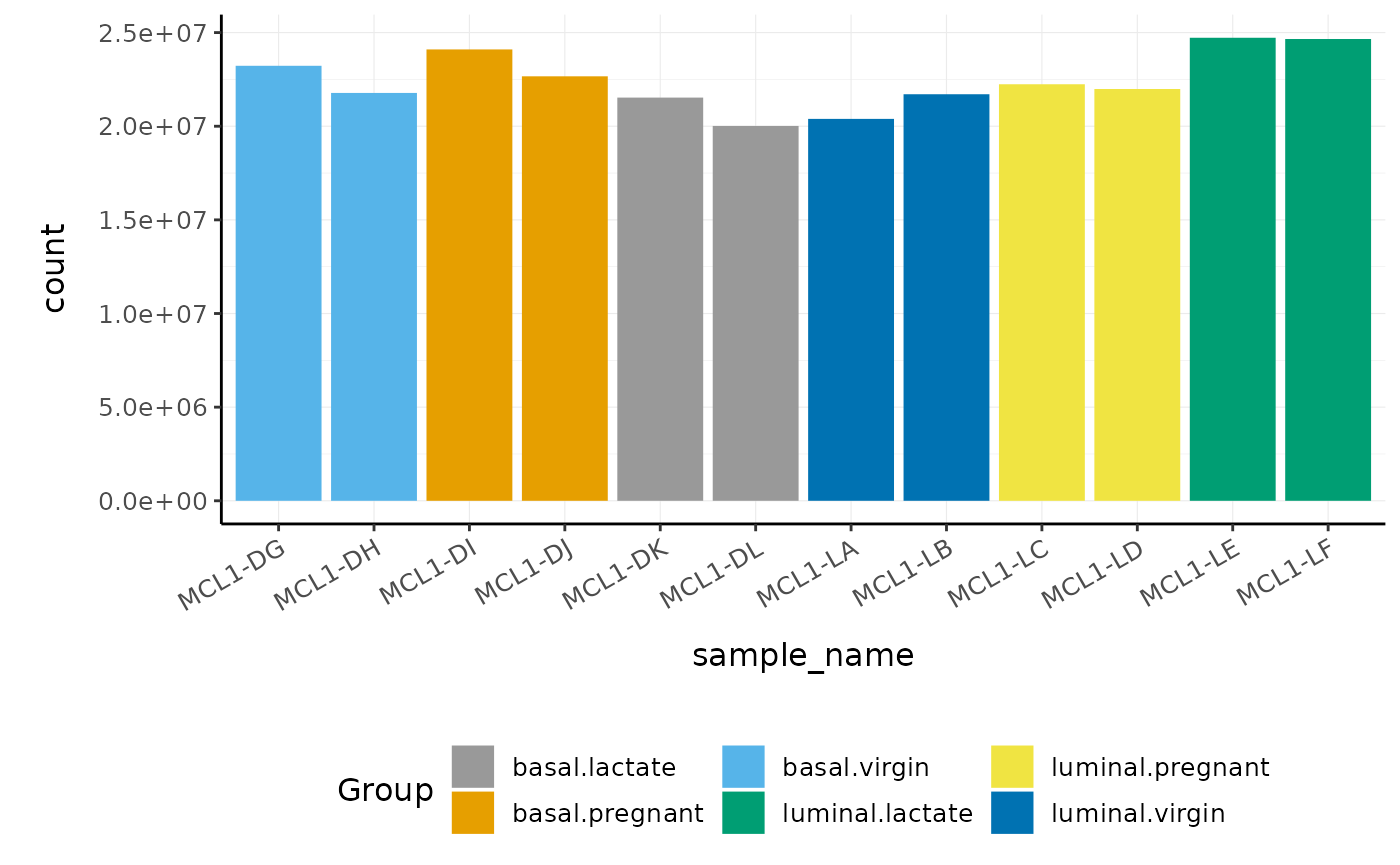
First, we can check how many reads we have for each sample.

counts_tt %>%
  group_by(sample_name) %>%
  summarise(total_reads = sum(counts))
#> # A tibble: 12 × 2
#>    sample_name total_reads
#>    <chr>             <dbl>
#>  1 MCL1-DG        23227641
#>  2 MCL1-DH        21777891
#>  3 MCL1-DI        24100765
#>  4 MCL1-DJ        22665371
#>  5 MCL1-DK        21529331
#>  6 MCL1-DL        20015386
#>  7 MCL1-LA        20392113
#>  8 MCL1-LB        21708152
#>  9 MCL1-LC        22241607
#> 10 MCL1-LD        21988240
#> 11 MCL1-LE        24723827
#> 12 MCL1-LF        24657293

We can also plot the library sizes as a barplot to see whether there are any major discrepancies between the samples more easily.

ggplot(counts_tt, aes(x = sample_name, weight = counts, fill = Group)) +
  geom_bar() +
  custom_theme

Scaling counts to normalise

We can use tidybulk function scale_abundance to scale counts, normalising for uninteresting differences between the samples, such as due to differences in sequencing depth or sample composition. Here we will use the default tidybulk normalisation method, edgeR’s trimmed mean of M values (TMM), (Robinson and Oshlack 2010).

# Scaling counts
counts_scaled <- counts_filtered %>% scale_abundance()
#> tidybulk says: the sample with largest library size MCL1-LB was chosen as reference for scaling

# take a look
counts_scaled
#> # A tibble: 191,628 × 15
#>    EntrezGeneID Length sample      counts sample_name symbol FileName SampleName
#>    <chr>         <dbl> <chr>        <dbl> <chr>       <chr>  <chr>    <chr>     
#>  1 497097         3634 MCL1-DG_BC…    438 MCL1-DG     Xkr4   MCL1.DG… MCL1.DG   
#>  2 497097         3634 MCL1-DH_BC…    300 MCL1-DH     Xkr4   MCL1.DH… MCL1.DH   
#>  3 497097         3634 MCL1-DI_BC…     65 MCL1-DI     Xkr4   MCL1.DI… MCL1.DI   
#>  4 497097         3634 MCL1-DJ_BC…    237 MCL1-DJ     Xkr4   MCL1.DJ… MCL1.DJ   
#>  5 497097         3634 MCL1-DK_BC…    354 MCL1-DK     Xkr4   MCL1.DK… MCL1.DK   
#>  6 497097         3634 MCL1-DL_BC…    287 MCL1-DL     Xkr4   MCL1.DL… MCL1.DL   
#>  7 497097         3634 MCL1-LA_BC…      0 MCL1-LA     Xkr4   MCL1.LA… MCL1.LA   
#>  8 497097         3634 MCL1-LB_BC…      0 MCL1-LB     Xkr4   MCL1.LB… MCL1.LB   
#>  9 497097         3634 MCL1-LC_BC…      0 MCL1-LC     Xkr4   MCL1.LC… MCL1.LC   
#> 10 497097         3634 MCL1-LD_BC…      0 MCL1-LD     Xkr4   MCL1.LD… MCL1.LD   
#> # … with 191,618 more rows, and 7 more variables: Group <chr>, CellType <chr>,
#> #   Status <chr>, .abundant <lgl>, TMM <dbl>, multiplier <dbl>,
#> #   counts_scaled <dbl>

After we run scale_abundance we should see some columns have been added at the end. The counts_scaled column contains the scaled counts.

We can visualise the difference of abundance distributions before and after scaling. As tidybulk output is compatible with tidyverse, we can simply pipe it into standard tidyverse functions such as filter, pivot_longer and ggplot. We can also take advantage of ggplot’s facet_wrap to easily create multiple plots.

counts_scaled %>%

  # Reshaping        
  pivot_longer(cols = c("counts", "counts_scaled"), names_to = "source", values_to = "abundance") %>%
    
  # Plotting
  ggplot(aes(x = sample_name, y = abundance + 1, fill = Group)) +
  geom_boxplot() +
  geom_hline(aes(yintercept = median(abundance + 1)), colour = "red") +
  facet_wrap(~source) +
  scale_y_log10() +
  custom_theme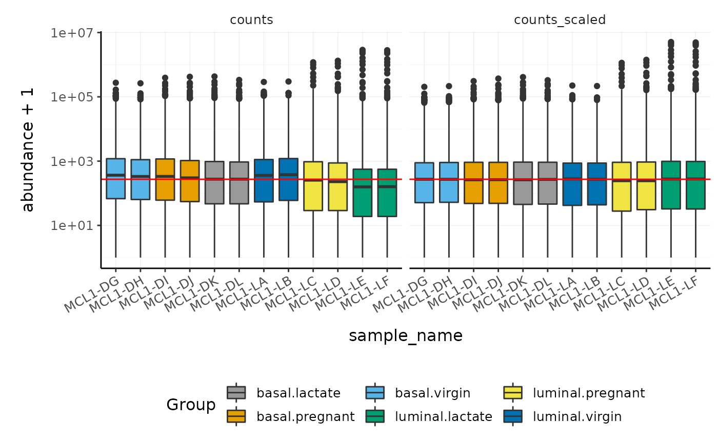

In this dataset the distributions of the counts are not very different to each other before scaling but scaling does make the distributions more similar. If we saw a sample with a very different distribution we may need to investigate it.

Exploratory analyses

Dimensionality reduction

We can use the reduce_dimensions function to calculate the dimensions and generate an MDS plot to check the quality of the data, outliers etc.

# Get principal components
counts_scal_MDS <-
  counts_scaled %>%
  reduce_dimensions(method = "MDS", scale=FALSE)
#> tidybulk says: to access the raw results do `attr(..., "internals")$MDS`
#> This message is displayed once per session.

This joins the result to the counts object.

# Take a look
counts_scal_MDS
#> # A tibble: 191,628 × 17
#>    EntrezGeneID Length sample      counts sample_name symbol FileName SampleName
#>    <chr>         <dbl> <chr>        <dbl> <chr>       <chr>  <chr>    <chr>     
#>  1 497097         3634 MCL1-DG_BC…    438 MCL1-DG     Xkr4   MCL1.DG… MCL1.DG   
#>  2 497097         3634 MCL1-DH_BC…    300 MCL1-DH     Xkr4   MCL1.DH… MCL1.DH   
#>  3 497097         3634 MCL1-DI_BC…     65 MCL1-DI     Xkr4   MCL1.DI… MCL1.DI   
#>  4 497097         3634 MCL1-DJ_BC…    237 MCL1-DJ     Xkr4   MCL1.DJ… MCL1.DJ   
#>  5 497097         3634 MCL1-DK_BC…    354 MCL1-DK     Xkr4   MCL1.DK… MCL1.DK   
#>  6 497097         3634 MCL1-DL_BC…    287 MCL1-DL     Xkr4   MCL1.DL… MCL1.DL   
#>  7 497097         3634 MCL1-LA_BC…      0 MCL1-LA     Xkr4   MCL1.LA… MCL1.LA   
#>  8 497097         3634 MCL1-LB_BC…      0 MCL1-LB     Xkr4   MCL1.LB… MCL1.LB   
#>  9 497097         3634 MCL1-LC_BC…      0 MCL1-LC     Xkr4   MCL1.LC… MCL1.LC   
#> 10 497097         3634 MCL1-LD_BC…      0 MCL1-LD     Xkr4   MCL1.LD… MCL1.LD   
#> # … with 191,618 more rows, and 9 more variables: Group <chr>, CellType <chr>,
#> #   Status <chr>, .abundant <lgl>, TMM <dbl>, multiplier <dbl>,
#> #   counts_scaled <dbl>, Dim1 <dbl>, Dim2 <dbl>

For plotting, we can select just the sample-wise information with pivot_sample.

# take a look
counts_scal_MDS %>% pivot_sample()
#> # A tibble: 12 × 12
#>    sample_name sample  FileName SampleName Group CellType Status .abundant   TMM
#>    <chr>       <chr>   <chr>    <chr>      <chr> <chr>    <chr>  <lgl>     <dbl>
#>  1 MCL1-DG     MCL1-D… MCL1.DG… MCL1.DG    basa… basal    virgin TRUE      1.25 
#>  2 MCL1-DH     MCL1-D… MCL1.DH… MCL1.DH    basa… basal    virgin TRUE      1.22 
#>  3 MCL1-DI     MCL1-D… MCL1.DI… MCL1.DI    basa… basal    pregn… TRUE      1.14 
#>  4 MCL1-DJ     MCL1-D… MCL1.DJ… MCL1.DJ    basa… basal    pregn… TRUE      1.09 
#>  5 MCL1-DK     MCL1-D… MCL1.DK… MCL1.DK    basa… basal    lacta… TRUE      1.05 
#>  6 MCL1-DL     MCL1-D… MCL1.DL… MCL1.DL    basa… basal    lacta… TRUE      1.11 
#>  7 MCL1-LA     MCL1-L… MCL1.LA… MCL1.LA    lumi… luminal  virgin TRUE      1.38 
#>  8 MCL1-LB     MCL1-L… MCL1.LB… MCL1.LB    lumi… luminal  virgin TRUE      1.38 
#>  9 MCL1-LC     MCL1-L… MCL1.LC… MCL1.LC    lumi… luminal  pregn… TRUE      1.02 
#> 10 MCL1-LD     MCL1-L… MCL1.LD… MCL1.LD    lumi… luminal  pregn… TRUE      0.924
#> 11 MCL1-LE     MCL1-L… MCL1.LE… MCL1.LE    lumi… luminal  lacta… TRUE      0.500
#> 12 MCL1-LF     MCL1-L… MCL1.LF… MCL1.LF    lumi… luminal  lacta… TRUE      0.504
#> # … with 3 more variables: multiplier <dbl>, Dim1 <dbl>, Dim2 <dbl>

We can now plot the reduced dimensions.

# MDS plot
counts_scal_MDS %>%
  pivot_sample() %>%
  ggplot(aes(x = Dim1, y = Dim2, colour = CellType, shape = Status)) +
  geom_point() +
  geom_text_repel(aes(label = sample_name), show.legend = FALSE) +
  custom_theme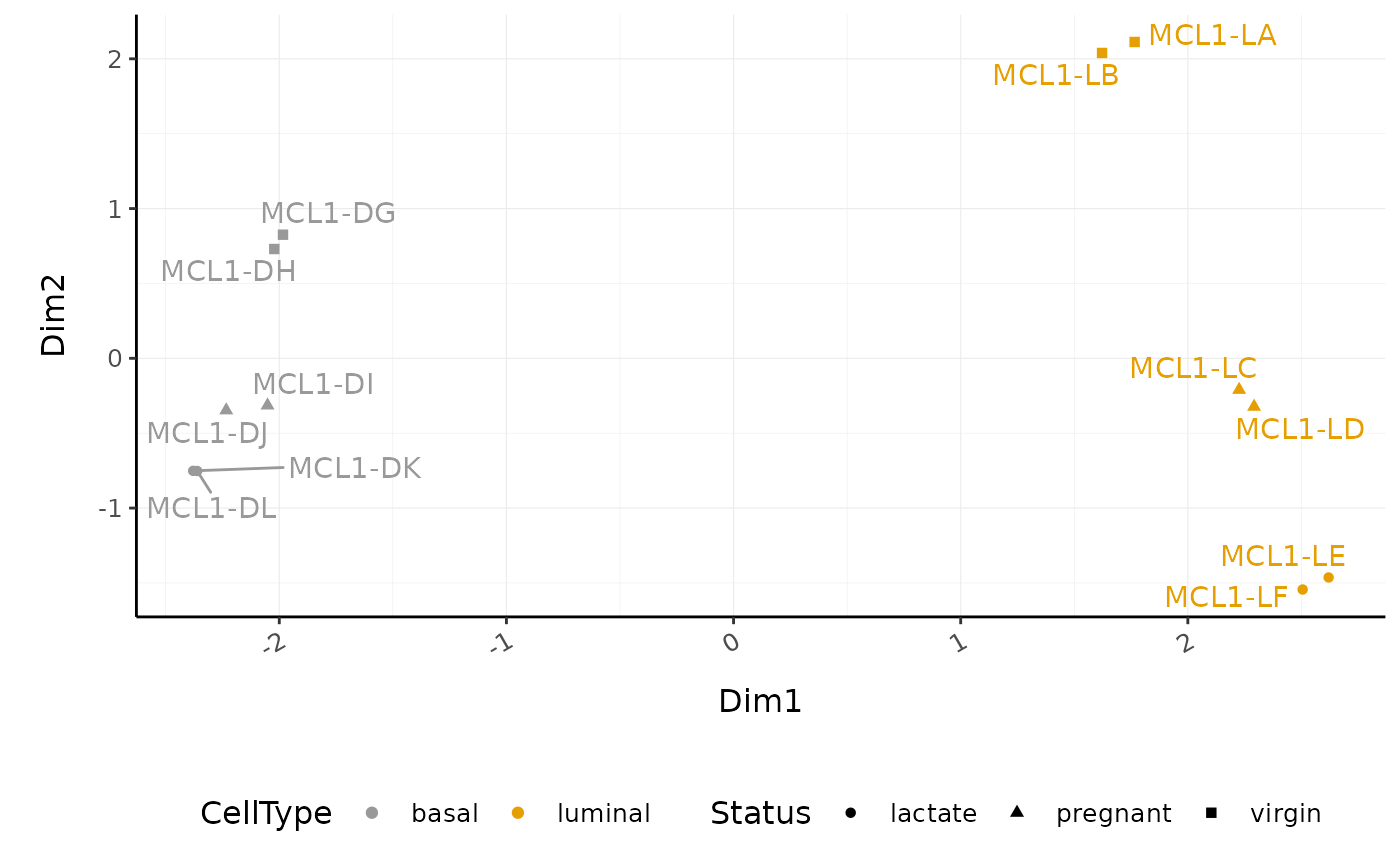

Hierarchical clustering with heatmaps

An alternative to principal component analysis for examining relationships between samples is using hierarchical clustering. tidybulk has a simple function we can use, keep_variable, to extract the most variable genes which we can then plot with tidyHeatmap.

counts_scal_MDS %>%

  # extract 500 most variable genes
  keep_variable(.abundance = counts_scaled, top = 500) %>%
  as_tibble() %>%

  # create heatmap
  heatmap(
    .column = sample_name,
    .row = EntrezGeneID,
    .value = counts_scaled,
    transform = log1p
  ) %>%
  add_tile(CellType) %>%
  add_tile(Status)
#> Getting the 500 most variable genes
#> tidyHeatmap says: (once per session) from release 1.7.0 the scaling is set to "none" by default. Please use scale = "row", "column" or "both" to apply scaling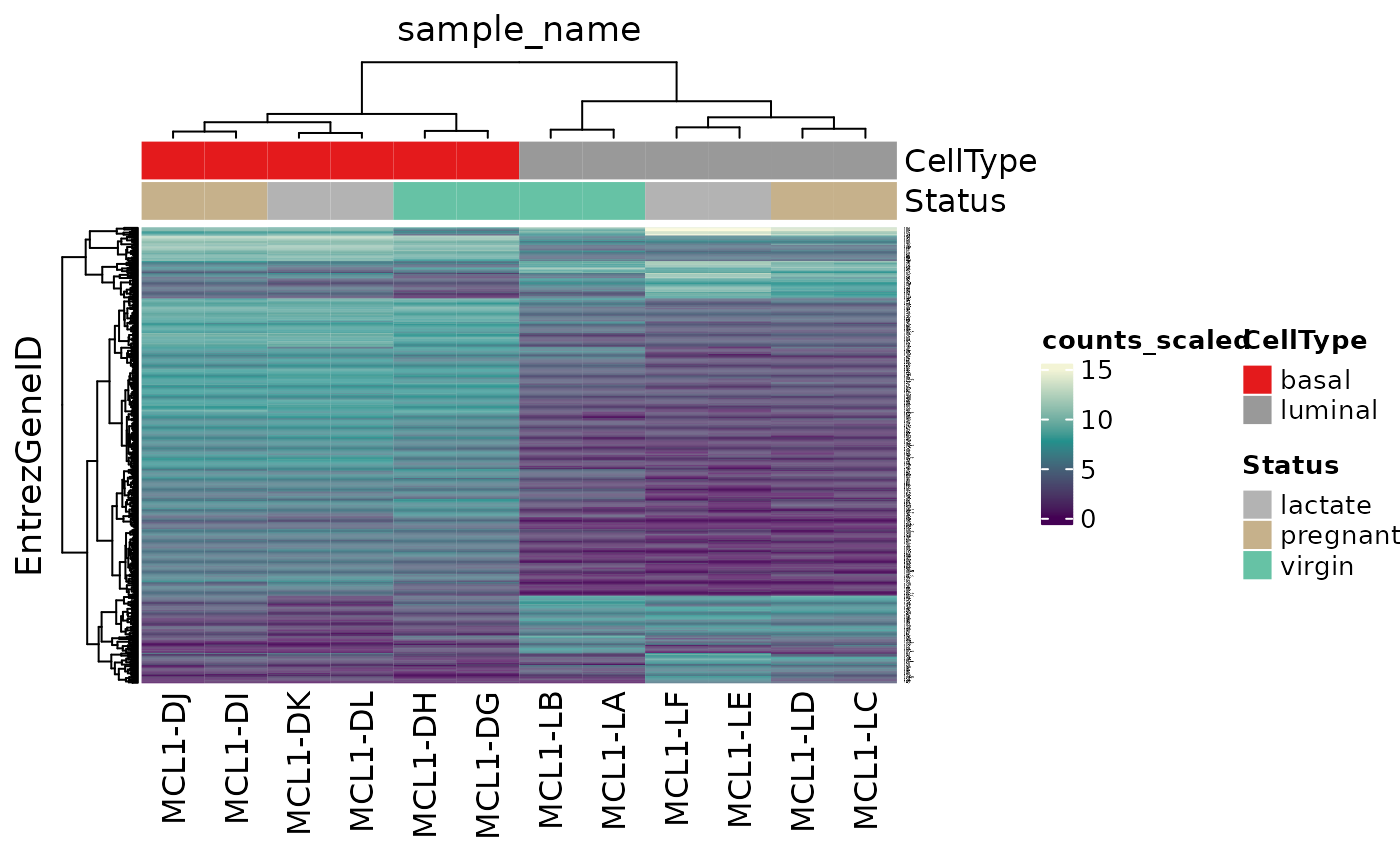

Differential expression

tidybulk integrates several popular methods for differential transcript abundance testing: the edgeR quasi-likelihood (Chen, Lun, and Smyth 2016) (tidybulk default method), edgeR likelihood ratio (McCarthy, Chen, and Smyth 2012), limma-voom (Law et al. 2014) and DESeq2 (Love, Huber, and Anders 2014). Here’s we’ll run limma-voom, the same method used in the original workshop that this material is based on.

We give test_differential_abundance our tidybulk counts object and a formula, specifying the column that contains our groups to be compared.

counts_de <- counts_scal_MDS %>%
    test_differential_abundance(~ 0 + Group,
                                 method = "limma_voom",
                                .contrasts =  c("Groupbasal.pregnant - Groupbasal.lactate"),
                                omit_contrast_in_colnames = TRUE)
#> =====================================
#> tidybulk says: All testing methods use raw counts, irrespective of if scale_abundance
#> or adjust_abundance have been calculated. Therefore, it is essential to add covariates
#> such as batch effects (if applicable) in the formula.
#> =====================================
#> tidybulk says: The design column names are "Groupbasal.lactate, Groupbasal.pregnant, Groupbasal.virgin, Groupluminal.lactate, Groupluminal.pregnant, Groupluminal.virgin"
#> 
#> tidybulk says: to access the raw results (fitted GLM) do `attr(..., "internals")$voom`
#> This message is displayed once per session.

This outputs the columns from each method such as log-fold change (logFC), false-discovery rate (adj.P.Val) and probability value (P.Value). logFC is log2(basal.pregnant/basal.lactate).

We can count the number of differentially expressed genes.

counts_de %>% 
    pivot_transcript() %>%
    mutate(signif=adj.P.Val<0.05) %>%
    summarise(Up=sum(signif & logFC>0), 
              Down=sum(signif & logFC<0),
              NotSig=sum(!signif))
#> # A tibble: 1 × 3
#>      Up  Down NotSig
#>   <int> <int>  <int>
#> 1  2702  2638  10629

Writing out the results

counts_de %>%
    pivot_transcript %>%
    write_tsv("de_results.tsv")

Plots after testing for differentially expressed

We’ll extract the symbols for a few top genes (by P value) to use in some of the plots we will make.

topgenes_symbols <-
  counts_de %>%
  pivot_transcript() %>%
  slice_min(P.Value, n=6) %>%
  pull(symbol)

MA plots

We can generate MA plots to visualise the results. MA plots enabel us to visualise the average expression (AveExpr) versus the fold change (logFC). Genes expressed at a high level are towards the right of the plot.

counts_de %>%
  pivot_transcript() %>%

  # Subset data
  mutate(significant = adj.P.Val < 0.05 & abs(logFC) >= 2) %>%
  mutate(transcript = ifelse(abs(logFC) >= 6, symbol, "")) %>%

  # Plot
  ggplot(aes(x = AveExpr, y = logFC, label = transcript)) +
  geom_point(aes(color = significant, size = significant, alpha = significant)) +
  geom_text_repel() +
  scale_color_manual(values = c("black", "#e11f28")) +
  scale_size_discrete(range = c(0, 2)) +
  custom_theme
#> Warning: Using size for a discrete variable is not advised.
#> Scale for 'colour' is already present. Adding another scale for 'colour',
#> which will replace the existing scale.
#> Warning: Using alpha for a discrete variable is not advised.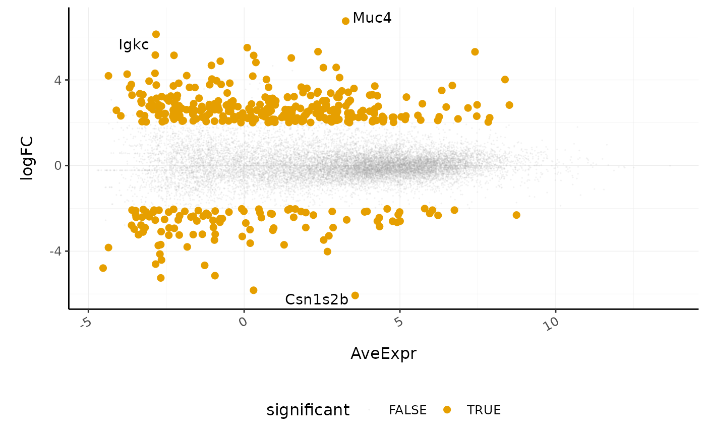

Volcano plots

Volcano plots are a useful genome-wide plot for checking that the analysis looks good. Volcano plots enable us to visualise the significance of change (p-value) versus the fold change (logFC). Highly significant genes are towards the top of the plot. We can also colour significant genes (e.g. genes with false-discovery rate < 0.05)

counts_de %>%
  pivot_transcript() %>%

  # Subset data
  mutate(significant = adj.P.Val < 0.05 & abs(logFC) >= 2) %>%
  mutate(symbol = ifelse(symbol %in% topgenes_symbols, as.character(symbol), "")) %>%

  # Plot
  ggplot(aes(x = logFC, y = P.Value, label = symbol)) +
  geom_point(aes(color = significant, size = significant, alpha = significant)) +
  geom_text_repel() +

  # Custom scales
  custom_theme +
  scale_y_continuous(trans = "log10_reverse") +
  scale_color_manual(values = c("black", "#e11f28")) +
  scale_size_discrete(range = c(0, 2))
#> Scale for 'colour' is already present. Adding another scale for 'colour',
#> which will replace the existing scale.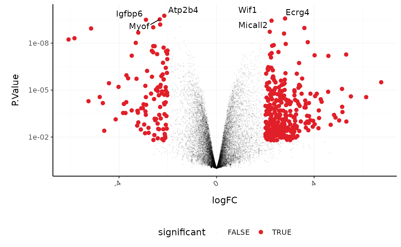

Stripcharts

We can use stripcharts to check if expression is consistent amongst replicates in the groups. Tidyverse faceting makes it easy to create a plot for each gene.

strip_chart <-
  counts_scaled %>%

  # extract counts for top differentially expressed genes
  filter(symbol %in% topgenes_symbols) %>%

  # make faceted stripchart
  ggplot(aes(x = Group, y = counts_scaled + 1, colour = Group, label = sample_name)) +
  geom_jitter() +
  facet_wrap(~symbol) +
  scale_y_log10() +
  custom_theme

strip_chart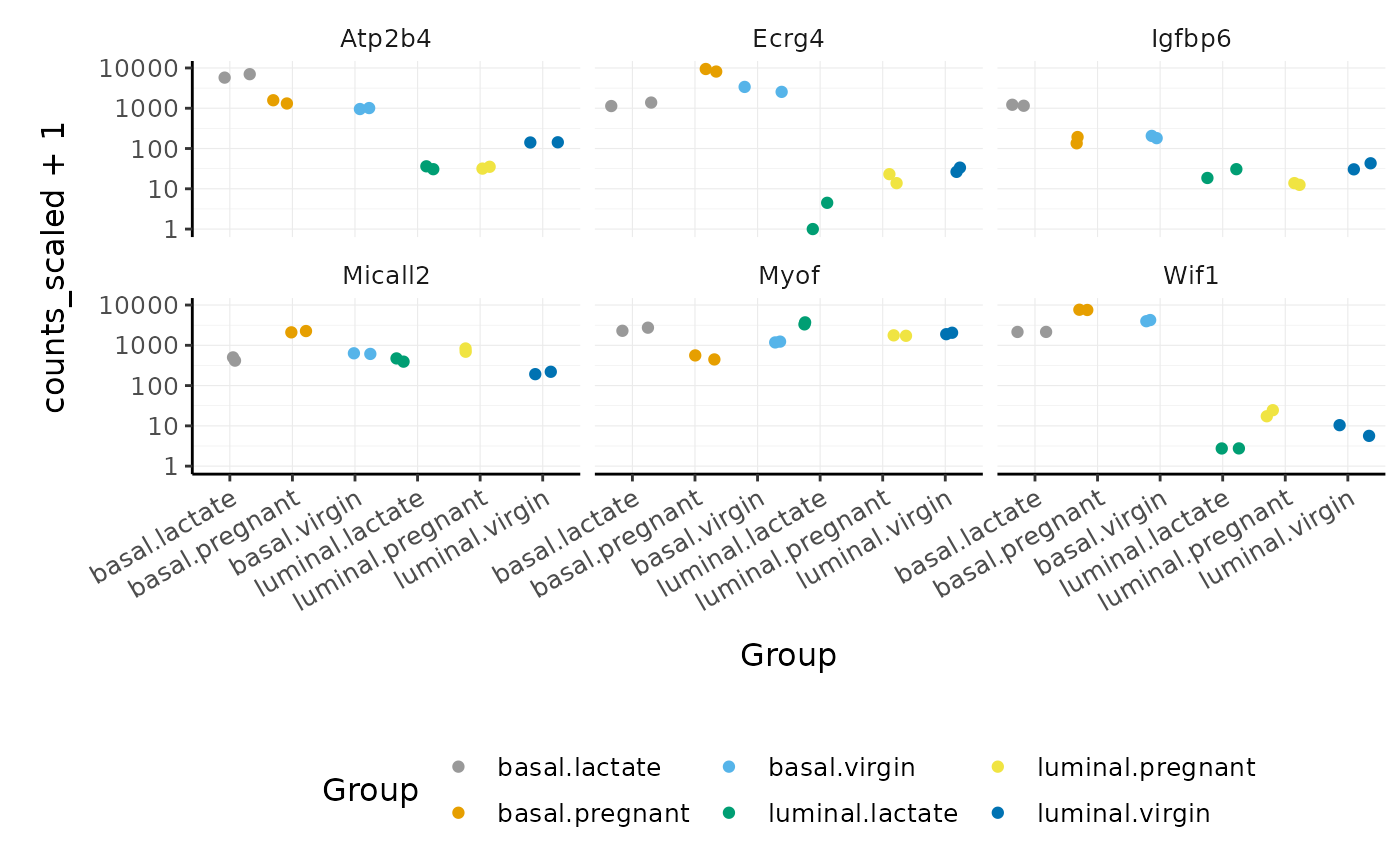

Interactive Plots

A really nice feature of using tidyverse and ggplot2 is that we can make interactive plots quite easily using the plotly package. This can be very useful for exploring what genes or samples are in the plots. We can make interactive plots directly from our ggplot2 object (strip_chart). Having label in the aes is useful to visualise the identifier of the data point (here the sample id) or other variables when we hover over the plot.

We can also specify which parameters from the aes we want to show up when we hover over the plot with tooltip.

strip_chart %>% ggplotly(tooltip = c("label", "y"))

Testing relative to a threshold (TREAT)

When there is a lot of differential expression, sometimes we may want to cut-off on a fold change threshold as well as a p-value threshold so that we follow up on the most biologically significant genes. There is a function called treat that performs this style of analysis correctly (McCarthy? and Smyth 2009). We simply need to specify a logFC cut-off with test_differential_abundance using test_above_log2_fold_change= and tidybulk will use treat to calculate the p-values taking into account the information about logFC. We’ll use a log2 fold change of 1 which is equivalent to a fold change of 2.

counts_de_treat <- counts_scal_MDS %>%
    test_differential_abundance(~ 0 + Group,
                                 method = "limma_voom",
                                .contrasts =  c("Groupbasal.pregnant - Groupbasal.lactate"),
                                omit_contrast_in_colnames = TRUE,
                                test_above_log2_fold_change = 1)
#> tidybulk says: The design column names are "Groupbasal.lactate, Groupbasal.pregnant, Groupbasal.virgin, Groupluminal.lactate, Groupluminal.pregnant, Groupluminal.virgin"

If we count the number of differentially expressed genes we can see there are less significant genes now.

counts_de_treat %>% 
    pivot_transcript() %>%
    mutate(signif=adj.P.Val<0.05) %>%
    summarise(Up=sum(signif & logFC>0), 
              Down=sum(signif & logFC<0),
              NotSig=sum(!signif))
#> # A tibble: 1 × 3
#>      Up  Down NotSig
#>   <int> <int>  <int>
#> 1    74    54  15841

Gene Set Testing

A common downstream procedure is gene set testing, which aims to understand which pathways/gene networks the differentially expressed genes are implicated in.

With tidybulk we can use test_gene_enrichment to perform gene set testing via EGSEA. EGSEA provides a choice of methods that can be used either individually or in combination to generate an ensemble score. Here we will demonstrate CAMERA, which is a good option for testing a very large number of gene sets, such as the MSigDB sets, as it is very fast. CAMERA is known as a competitive gene set test, however it has the advantage that it can take into account inter-gene correlation within each gene set (Wu and Smyth 2012).

EGSEA also provide collections of gene sets from the Broad Institute’s Molecular Signatures Database (MSigDB) for human, mouse and rat. The c2 gene sets contain >5000 curated gene sets collected from a variety of places: BioCarta, KEGG, Pathway Interaction Database, Reactome as well as some published studies.

counts_egsea <- counts_scaled %>%
    test_gene_enrichment(.entrez=EntrezGeneID, 
                         .abundance=counts_scaled, 
                         .formula=~ 0 + Group, 
                         .contrasts =  c("Groupbasal.pregnant - Groupbasal.lactate"), 
                         species="mouse", 
                         methods="camera",
                         gene_sets="c2")
#> [1] "Loading MSigDB Gene Sets ... "
#> [1] "Loaded gene sets for the collection c2 ..."
#> [1] "Indexed the collection c2 ..."
#> [1] "Created annotation for the collection c2 ..."
#> ##------ Mon Jun 27 20:12:10 2022 ------##
#> ##------ Mon Jun 27 20:12:12 2022 ------##
#> ##------ Mon Jun 27 20:12:12 2022 ------##
#> ##------ Mon Jun 27 20:12:25 2022 ------##

The output is a tibble containing each gene set tested with P values and other information. A HTML report is also produced containing summary plots.

counts_egsea
#> # A tibble: 4,725 × 11
#>    data_base pathway       web_page  p.value NGenes Direction    p.adj avg.logfc
#>    <chr>     <chr>         <chr>       <dbl>  <dbl> <chr>        <dbl>     <dbl>
#>  1 c2        REACTOME_3_U… https:/… 3.36e-25    128 Up        1.21e-21     0.674
#>  2 c2        REACTOME_PEP… https:/… 5.11e-25    102 Up        1.21e-21     0.688
#>  3 c2        KEGG_RIBOSOME https:/… 1.05e-24    102 Up        1.65e-21     0.695
#>  4 c2        REACTOME_TRA… https:/… 4.43e-23    176 Up        5.23e-20     0.658
#>  5 c2        REACTOME_SRP… https:/… 1.68e-22    130 Up        1.59e-19     0.679
#>  6 c2        REACTOME_NON… https:/… 2.37e-21    132 Up        1.87e-18     0.686
#>  7 c2        REACTOME_INF… https:/… 3.50e-21    122 Up        2.36e-18     0.693
#>  8 c2        REACTOME_FOR… https:/… 5.17e-17     56 Up        3.05e-14     0.667
#>  9 c2        REACTOME_INF… https:/… 8.85e-17    169 Up        4.65e-14     0.691
#> 10 c2        REACTOME_ACT… https:/… 1.71e-16     67 Up        8.10e-14     0.654
#> # … with 4,715 more rows, and 3 more variables: avg.logfc.dir <dbl>,
#> #   direction <dbl>, significance <dbl>

Automatic bibliography

Tidybulk provides a handy function called get_bibliography that keeps track of the references for the methods used in your tidybulk workflow. The references are in BibTeX format and can be imported into your reference manager.

get_bibliography(counts_egsea)
#>  @Article{tidybulk,
#>   title = {tidybulk: an R tidy framework for modular transcriptomic data analysis},
#>   author = {Stefano Mangiola and Ramyar Molania and Ruining Dong and Maria A. Doyle & Anthony T. Papenfuss},
#>   journal = {Genome Biology},
#>   year = {2021},
#>   volume = {22},
#>   number = {42},
#>   url = {https://genomebiology.biomedcentral.com/articles/10.1186/s13059-020-02233-7},
#>   }
#> @article{wickham2019welcome,
#>   title={Welcome to the Tidyverse},
#>   author={Wickham, Hadley and Averick, Mara and Bryan, Jennifer and Chang, Winston and McGowan, Lucy D'Agostino and Francois, Romain and Grolemund, Garrett and Hayes, Alex and Henry, Lionel and Hester, Jim and others},
#>   journal={Journal of Open Source Software},
#>   volume={4},
#>   number={43},
#>   pages={1686},
#>   year={2019}
#>  }
#> @article{robinson2010edger,
#>   title={edgeR: a Bioconductor package for differential expression analysis of digital gene expression data},
#>   author={Robinson, Mark D and McCarthy, Davis J and Smyth, Gordon K},
#>   journal={Bioinformatics},
#>   volume={26},
#>   number={1},
#>   pages={139--140},
#>   year={2010},
#>   publisher={Oxford University Press}
#>  }
#> @article{robinson2010scaling,
#>   title={A scaling normalization method for differential expression analysis of RNA-seq data},
#>   author={Robinson, Mark D and Oshlack, Alicia},
#>   journal={Genome biology},
#>   volume={11},
#>   number={3},
#>   pages={1--9},
#>   year={2010},
#>   publisher={BioMed Central}
#>  }
#> @article{alhamdoosh2017combining,
#>   title={Combining multiple tools outperforms individual methods in gene set enrichment analyses},
#>   author={Alhamdoosh, Monther and Ng, Milica and Wilson, Nicholas J and Sheridan, Julie M and Huynh, Huy and Wilson, Michael J and Ritchie, Matthew E},
#>   journal={Bioinformatics},
#>   volume={33},
#>   number={3},
#>   pages={414--424},
#>   year={2017},
#>   publisher={Oxford University Press}
#>   }
#> @article{liberzon2011molecular,
#>   title={Molecular signatures database (MSigDB) 3.0},
#>   author={Liberzon, Arthur and Subramanian, Aravind and Pinchback, Reid and Thorvaldsdottir, Helga and Tamayo, Pablo and Mesirov, Jill P},
#>   journal={Bioinformatics},
#>   volume={27},
#>   number={12},
#>   pages={1739--1740},
#>   year={2011},
#>   publisher={Oxford University Press}
#>  }
#> @article{Wu2012,
#>   doi = {10.1093/nar/gks461},
#>   url = {https://doi.org/10.1093/nar/gks461},
#>   year = {2012},
#>   month = may,
#>   publisher = {Oxford University Press ({OUP})},
#>   volume = {40},
#>   number = {17},
#>   pages = {e133--e133},
#>   author = {Di Wu and Gordon K. Smyth},
#>   title = {Camera: a competitive gene set test accounting for inter-gene correlation},
#>   journal = {Nucleic Acids Research}
#> }

Contributing

If you want to suggest improvements for this material or ask questions, you can do so as described here.

Reproducibility

Record package and version information with sessionInfo

sessionInfo()
#> R version 4.2.0 (2022-04-22)
#> Platform: x86_64-pc-linux-gnu (64-bit)
#> Running under: Ubuntu 20.04.4 LTS
#> 
#> Matrix products: default
#> BLAS:   /usr/lib/x86_64-linux-gnu/openblas-pthread/libblas.so.3
#> LAPACK: /usr/lib/x86_64-linux-gnu/openblas-pthread/liblapack.so.3
#> 
#> locale:
#>  [1] LC_CTYPE=en_US.UTF-8       LC_NUMERIC=C              
#>  [3] LC_TIME=en_US.UTF-8        LC_COLLATE=en_US.UTF-8    
#>  [5] LC_MONETARY=en_US.UTF-8    LC_MESSAGES=en_US.UTF-8   
#>  [7] LC_PAPER=en_US.UTF-8       LC_NAME=C                 
#>  [9] LC_ADDRESS=C               LC_TELEPHONE=C            
#> [11] LC_MEASUREMENT=en_US.UTF-8 LC_IDENTIFICATION=C       
#> 
#> attached base packages:
#> [1] stats4    stats     graphics  grDevices utils     datasets  methods  
#> [8] base     
#> 
#> other attached packages:
#>  [1] tidybulk_1.8.0       tidyHeatmap_1.8.1    EGSEA_1.24.0        
#>  [4] pathview_1.36.0      topGO_2.48.0         SparseM_1.81        
#>  [7] GO.db_3.15.0         graph_1.74.0         AnnotationDbi_1.58.0
#> [10] IRanges_2.30.0       S4Vectors_0.34.0     gage_2.46.0         
#> [13] Biobase_2.56.0       BiocGenerics_0.42.0  ggrepel_0.9.1       
#> [16] plotly_4.10.0        ggplot2_3.3.6        stringr_1.4.0       
#> [19] readr_2.1.2          tidyr_1.2.0          dplyr_1.0.9         
#> [22] tibble_3.1.7        
#> 
#> loaded via a namespace (and not attached):
#>   [1] utf8_1.2.2                  tidyselect_1.1.2           
#>   [3] RSQLite_2.2.14              htmlwidgets_1.5.4          
#>   [5] grid_4.2.0                  BiocParallel_1.30.3        
#>   [7] R2HTML_2.3.3                munsell_0.5.0              
#>   [9] ScaledMatrix_1.4.0          preprocessCore_1.58.0      
#>  [11] codetools_0.2-18            mutoss_0.1-12              
#>  [13] ragg_1.2.2                  DT_0.23                    
#>  [15] KEGGdzPathwaysGEO_1.34.0    withr_2.5.0                
#>  [17] colorspace_2.0-3            highr_0.9                  
#>  [19] knitr_1.39                  SingleCellExperiment_1.18.0
#>  [21] labeling_0.4.2              MatrixGenerics_1.8.1       
#>  [23] Rdpack_2.3.1                KEGGgraph_1.56.0           
#>  [25] org.Rn.eg.db_3.15.0         GenomeInfoDbData_1.2.8     
#>  [27] mnormt_2.1.0                hwriter_1.3.2.1            
#>  [29] farver_2.1.0                bit64_4.0.5                
#>  [31] rhdf5_2.40.0                rprojroot_2.0.3            
#>  [33] vctrs_0.4.1                 generics_0.1.2             
#>  [35] TH.data_1.1-1               xfun_0.31                  
#>  [37] doParallel_1.0.17           R6_2.5.1                   
#>  [39] GenomeInfoDb_1.32.2         clue_0.3-61                
#>  [41] rsvd_1.0.5                  locfit_1.5-9.5             
#>  [43] bitops_1.0-7                rhdf5filters_1.8.0         
#>  [45] cachem_1.0.6                DelayedArray_0.22.0        
#>  [47] vroom_1.5.7                 scales_1.2.0               
#>  [49] multcomp_1.4-19             gtable_0.3.0               
#>  [51] beachmat_2.12.0             org.Mm.eg.db_3.15.0        
#>  [53] sandwich_3.0-2              rlang_1.0.3                
#>  [55] systemfonts_1.0.4           GlobalOptions_0.1.2        
#>  [57] splines_4.2.0               lazyeval_0.2.2             
#>  [59] PADOG_1.38.0                yaml_2.3.5                 
#>  [61] crosstalk_1.2.0             tools_4.2.0                
#>  [63] ellipsis_0.3.2              gplots_3.1.3               
#>  [65] jquerylib_0.1.4             RColorBrewer_1.1-3         
#>  [67] HTMLUtils_0.1.8             TFisher_0.2.0              
#>  [69] Rcpp_1.0.8.3                sparseMatrixStats_1.8.0    
#>  [71] zlibbioc_1.42.0             purrr_0.3.4                
#>  [73] RCurl_1.98-1.7              viridis_0.6.2              
#>  [75] GetoptLong_1.0.5            hgu133plus2.db_3.13.0      
#>  [77] zoo_1.8-10                  cluster_2.1.3              
#>  [79] SummarizedExperiment_1.26.1 fs_1.5.2                   
#>  [81] magrittr_2.0.3              data.table_1.14.2          
#>  [83] circlize_0.4.15             mvtnorm_1.1-3              
#>  [85] matrixStats_0.62.0          patchwork_1.1.1            
#>  [87] hms_1.1.1                   evaluate_0.15              
#>  [89] GSVA_1.44.2                 xtable_1.8-4               
#>  [91] globaltest_5.50.0           XML_3.99-0.10              
#>  [93] hgu133a.db_3.13.0           gridExtra_2.3              
#>  [95] shape_1.4.6                 EGSEAdata_1.24.0           
#>  [97] compiler_4.2.0              safe_3.36.0                
#>  [99] KernSmooth_2.23-20          crayon_1.5.1               
#> [101] htmltools_0.5.2             tzdb_0.3.0                 
#> [103] DBI_1.1.3                   ComplexHeatmap_2.12.0      
#> [105] MASS_7.3-57                 Matrix_1.4-1               
#> [107] cli_3.3.0                   rbibutils_2.2.8            
#> [109] parallel_4.2.0              metap_1.8                  
#> [111] qqconf_1.2.3                GenomicRanges_1.48.0       
#> [113] pkgconfig_2.0.3             pkgdown_2.0.5              
#> [115] sn_2.0.2                    numDeriv_2016.8-1.1        
#> [117] foreach_1.5.2               annotate_1.74.0            
#> [119] bslib_0.3.1                 rngtools_1.5.2             
#> [121] multtest_2.52.0             XVector_0.36.0             
#> [123] doRNG_1.8.2                 digest_0.6.29              
#> [125] Biostrings_2.64.0           rmarkdown_2.14             
#> [127] dendextend_1.15.2           edgeR_3.38.1               
#> [129] DelayedMatrixStats_1.18.0   GSEABase_1.58.0            
#> [131] curl_4.3.2                  gtools_3.9.2.2             
#> [133] rjson_0.2.21                GSA_1.03.2                 
#> [135] lifecycle_1.0.1             nlme_3.1-158               
#> [137] jsonlite_1.8.0              Rhdf5lib_1.18.2            
#> [139] desc_1.4.1                  viridisLite_0.4.0          
#> [141] limma_3.52.2                fansi_1.0.3                
#> [143] pillar_1.7.0                lattice_0.20-45            
#> [145] KEGGREST_1.36.2             fastmap_1.1.0              
#> [147] httr_1.4.3                  plotrix_3.8-2              
#> [149] survival_3.3-1              glue_1.6.2                 
#> [151] png_0.1-7                   iterators_1.0.14           
#> [153] bit_4.0.4                   Rgraphviz_2.40.0           
#> [155] stringi_1.7.6               sass_0.4.1                 
#> [157] HDF5Array_1.24.1            blob_1.2.3                 
#> [159] textshaping_0.3.6           org.Hs.eg.db_3.15.0        
#> [161] BiocSingular_1.12.0         caTools_1.18.2             
#> [163] memoise_2.0.1               mathjaxr_1.6-0             
#> [165] irlba_2.3.5

References

Chen, Yunshun, Aaron TL Lun, and Gordon K Smyth. 2016. “From Reads to Genes to Pathways: Differential Expression Analysis of RNA-Seq Experiments Using Rsubread and the edgeR Quasi-Likelihood Pipeline.” F1000Research 5.

Law, Charity W, Monther Alhamdoosh, Shian Su, Xueyi Dong, Luyi Tian, Gordon K Smyth, and Matthew E Ritchie. 2016. “RNA-Seq Analysis Is Easy as 1-2-3 with Limma, Glimma and edgeR.” F1000Research 5.

Law, Charity W, Yunshun Chen, Wei Shi, and Gordon K Smyth. 2014. “Voom: Precision Weights Unlock Linear Model Analysis Tools for RNA-Seq Read Counts.” Genome Biology 15 (2): R29.

Love, Michael I, Wolfgang Huber, and Simon Anders. 2014. “Moderated Estimation of Fold Change and Dispersion for RNA-Seq Data with DESeq2.” Genome Biology 15 (12): 550.

Mangiola, Stefano, Ramyar Molania, Ruining Dong, Maria A. Doyle, and Anthony T. Papenfuss. 2021. “Tidybulk: An r Tidy Framework for Modular Transcriptomic Data Analysis.” Genome Biology 22 (1). https://doi.org/10.1186/s13059-020-02233-7.

Mangiola, Stefano, and Anthony T Papenfuss. 2020. “tidyHeatmap: An r Package for Modular Heatmap Production Based on Tidy Principles.” Journal of Open Source Software 5 (52): 2472.

McCarthy, Davis J, Yunshun Chen, and Gordon K Smyth. 2012. “Differential Expression Analysis of Multifactor RNA-Seq Experiments with Respect to Biological Variation.” Nucleic Acids Research 40 (10): 4288–97.

Robinson, Mark D, and Alicia Oshlack. 2010. “A Scaling Normalization Method for Differential Expression Analysis of RNA-Seq Data.” Genome Biology 11 (3): 1–9.

Wickham, Hadley et al. 2014. “Tidy Data.” Journal of Statistical Software 59 (10): 1–23.

Wickham, Hadley, Mara Averick, Jennifer Bryan, Winston Chang, Lucy D’Agostino McGowan, Romain François, Garrett Grolemund, et al. 2019. “Welcome to the Tidyverse.” Journal of Open Source Software 4 (43): 1686.

<maria.doyle at petermac.org>↩︎
<mangiola.s at wehi.edu.au>↩︎

Maria Doyle, Peter MacCallum Cancer Centre¹

Stefano Mangiola, Walter and Eliza Hall Institute²

27 June 2022

Introduction

Acknowledgements

Setting up the data

Mouse mammary gland dataset

Importing the data

Format the data

Adding annotation

Convert counts to tidybulk tibble

Filtering lowly expressed genes

Quality control

Library size and distribution plots

Scaling counts to normalise

Exploratory analyses

Dimensionality reduction

Hierarchical clustering with heatmaps

Differential expression

Writing out the results

Plots after testing for differentially expressed

MA plots

Volcano plots

Stripcharts

Interactive Plots

Testing relative to a threshold (TREAT)

Gene Set Testing

Automatic bibliography

Contributing

Reproducibility

References

RNAseq-R-tidyverse

Maria Doyle, Peter MacCallum Cancer Centre1

Stefano Mangiola, Walter and Eliza Hall Institute2

27 June 2022

Introduction

Acknowledgements

Setting up the data

Mouse mammary gland dataset

Importing the data

Format the data

Adding annotation

Convert counts to tidybulk tibble

Filtering lowly expressed genes

Quality control

Library size and distribution plots

Scaling counts to normalise

Exploratory analyses

Dimensionality reduction

Hierarchical clustering with heatmaps

Differential expression

Writing out the results

Plots after testing for differentially expressed

MA plots

Volcano plots

Stripcharts

Interactive Plots

Testing relative to a threshold (TREAT)

Gene Set Testing

Automatic bibliography

Contributing

Reproducibility

References

Maria Doyle, Peter MacCallum Cancer Centre¹

Stefano Mangiola, Walter and Eliza Hall Institute²